Introduction
In this article we will demonstrate practical work in Statistica software, specifically detecting the influence of individual factors on the behavior of laboratory rats in a maze.
Data
We have three strains of rats whose general ability to successfully navigate a maze can be described as good, inconsistent, or poor. Four rats from each strain were raised in a stimulating environment and four in a restricted environment. The goal is to determine whether strain, environment, or both have an effect on the number of errors a rat makes in the maze. The data for this example can be found in File / Open Examples / Datasets / Rats.sta.
Analysis – procedure
Feel free to click through this example step by step with us.
After loading the data in Statistica, we choose: Statistics / ANOVA / General ANOVA/MANOVA dialog – Factorial ANOVA (as the analysis type); in the Method field we leave the specification set to Quick specs. We click OK. The ANOVA/MANOVA Factorial ANOVA dialog appears. We click the Variables button and select Errors as the dependent variable and Strain and Environment as categorical predictors. We click OK twice to reach the ANOVA Results dialog. This dialog offers plenty of options for choosing a wide variety of results. They are organized across eight tabs.
If eight tabs are not enough for you, you can switch to an even more comprehensive results dialog by pressing the More results button.
You can return to the original results dialog by pressing the Less button. Now, by clicking the All effects/graphs button on the Quick tab, we display the Table of all effects dialog. Both effects (Environment and Strain) are marked as significant (they are marked with an asterisk *), but the interaction effect (Environment*Strain) is not significant.
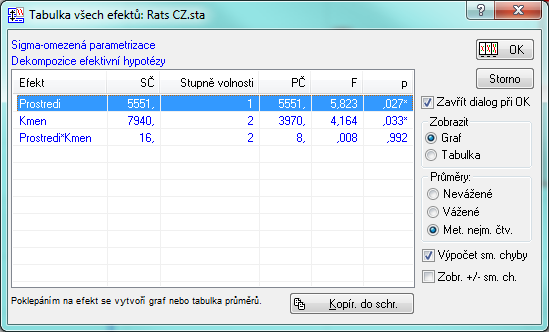
Note: In practice, after these findings we would probably redefine the model without interactions, i.e. in the General ANOVA/MANOVA menu dialog we would not choose Factorial ANOVA but Main effects ANOVA.
However, because the influence of the interactions on the result is negligible, and since it will also let us show how to recognize non-significant interactions from a graph, we will continue with the model that includes interactions.
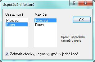
In analysis of variance, marginal means are one of the main characteristics that tell us something about the dataset. They can be easily computed and displayed, for example by selecting (clicking) the interaction effect (Environment*Strain) in the table above (Table of all effects) and clicking OK. The Arrangement of factors dialog appears, in which we specify what the resulting graph will look like. For the purposes of this example, we set Strain in the x-axis, upper list and Environment in the Line pattern list:
By clicking OK we create the corresponding graph. We can clearly see that rats raised in a restricted environment made more errors than rats raised in a stimulating environment, regardless of strain. At the same time, rats with a poor ability to navigate the maze made the most errors, while the clever rats made the fewest.
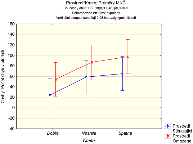
The graph also shows the non-significance of the interactions, since the two curves are parallel.
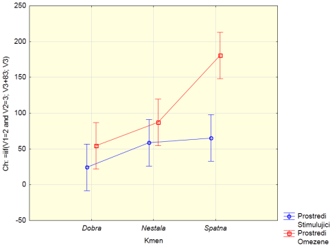
Note: For illustration, let us also mention cases of what a graph revealing significant interactions would look like. This could be a graph in which the individual lines connecting the factor means cross, or in which the mean value of the dependent variable differs significantly for a particular combination of factors. In such cases, we would probably be dealing with a statistically significant interaction. The second case described is illustrated by the graph.
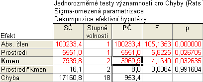
The ANOVA results can also be displayed in table form by clicking the All effects button on the Quick tab. Significant effects are highlighted in red.
Post-hoc tests
As already mentioned, this analysis revealed a significant effect of the factors Environment and Strain. Let us emphasize, however, that the significance test tells us nothing about which of the groups of rats differs significantly from the others in the number of errors. To find this out, we can run post-hoc tests. We click the More results button and then the Post-hoc tab:
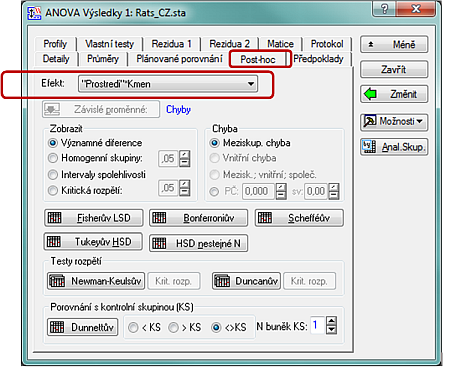
In the Effect field we choose Strain so that we can compare the marginal means for this effect. By clicking the Scheffé button, the results of the Scheffé test are displayed in the table:
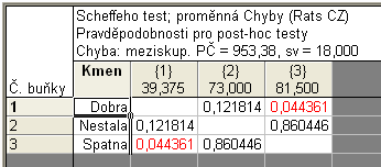
This table shows the statistical significance of the differences in means for all pairs of rat groups. As can be seen, only the difference between the 1st and 3rd group, i.e. between the dull and the clever rats, is statistically significant at the 0.05 significance level. We can therefore conclude that only the dull rats made significantly more errors than the clever rats, whereas the average rats do not differ significantly from the other two groups.
Assumptions
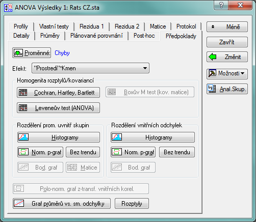
We now have the results of the analysis of variance itself. But as the picture of the electronic nurse of our studied rats suggests, more clicking still awaits us. Of course, we need to test the assumptions under which the ANOVA method can be applied. We therefore switch to the Assumptions tab:
Normality
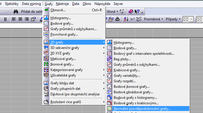
The first assumption of analysis of variance that we verify is the normality of the observed samples. We therefore need to verify the assumption that the distribution of the dependent variable within each group is normal. To assess the type of distribution of the dependent variable, we can use, for example, normal probability plots, which are available directly on the Assumptions tab. Or via the menu Graphs / 2D Graphs / Normal probability plots… On the Graphs tab, however, you can tick the Shapiro–Wilk test as an addition to the output, which lets you test the null hypothesis about the normality of a particular sample and thus support the visual estimate.
Note: Normal probability plots serve as a visual aid when testing the normality assumption – the closer the points in the plot lie to the plotted straight line, the closer we are to the normal distribution. We should watch out mainly for any systematic deviation from the line, such as an S-shaped pattern.
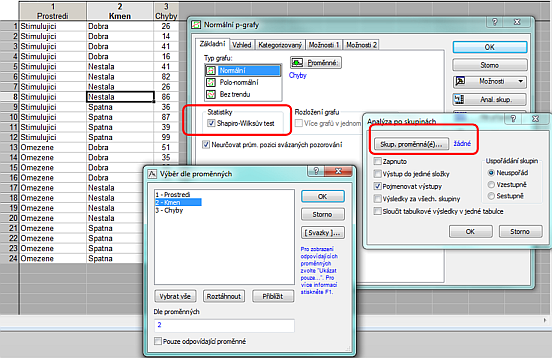
If normality were to be assessed at the level of a single factor, it is easy to break the grouped sample down by using the Analysis by groups tab:
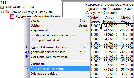
With multiple factors and interactions it is no longer entirely simple to cover all the options; moreover, the individual groups then contain very little data, so it is better to test the normality assumption after estimating the model parameters, directly on its residuals. We switch to the Residuals tab, where we have rich options for looking at this vector. We can either look at the normality of the residuals directly by clicking Normal probability plot of residuals, or we can do it in two steps: first we generate the residuals into a Statistica workbook by clicking the Predicted & residuals button. In the Statistica workbook we then set the residuals table as the active input:
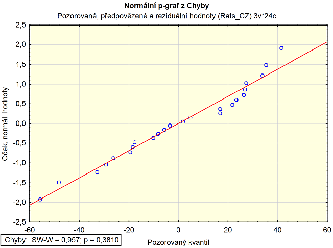
We again display the Normal probability plot (via the Graphs menu) and the results of the Shapiro-Wilk test, which confirm (p = 0.3810) the visual estimate of the data, namely that we do not reject the null hypothesis about the residuals.
You can also use a whole range of graphs available on the Residuals tab directly within the ANOVA analysis.
Homogeneity of variances
Another assumption is the homogeneity of variances between groups. Statistica provides several tests of this assumption in the Homogeneity of variances/covariances group on the Assumptions tab. Given the normality of the data, for the purposes of this example we use Levene's test (ANOVA).
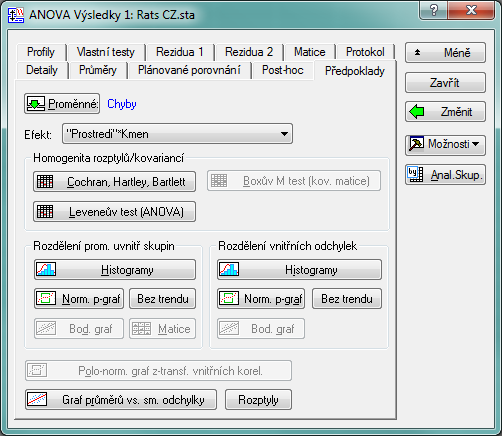
The table of results of this test shown below does not display any values indicating that the variance in the individual groups is statistically significantly different (i.e. the condition of homogeneity of variances is satisfied).
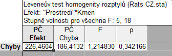
We have thus verified the assumptions for applying analysis of variance methods to the rat data. You can learn more about the options in the ANOVA results dialog in our specialized Analysis of Variance course.
Conclusion
As the results of the analysis suggest, we can say with high probability that both the factor of genetic disposition and the upbringing environment have a significant effect on the rats' ability to navigate the maze.